Common Outcome-Based Algorithmic Fairness Metrics
Data Science Ethics

algorithmic fairness metrics from Machines Gone Wrong.
Algorithms are becoming an increasingly ubiquitous component of decision-making with high moral stakes, such as loan and mortgage approval, governmental aid allocations, health insurance claim approval, and US bail and sentencing procedures. With the growing use of algorithms in settings with high moral stakes, there has also been a growing concern about algorithmic fairness, or more specifically, whether an algorithm used to make decisions in such settings is (un)fair.
Many statistical metrics have been developed to assess whether a given algorithm is (un)fair. Since 2022, I have been interested in these measures and how they track with discussions of fairness and justice coming from Philosophy – a field which has been theorizing about fairness and justice for more than two millennia. However, when doing research on statistical metrics of fairness, I realized that the definitions of such metrics tend to be scattered across multiple papers, making it difficult to understand how different metrics compare (or motivate) one another.
In this notebook, I provide an overview of common algorithmic fairness metrics coming from Statistics and draw comparison between the described metrics. For simplicity, this notebook focuses on outcome-based measures of fairness (i.e., metrics that evaluate an algorithm for fairness using its outputted predictions). In a future notebook, I hope to delve into more procedural-based algorithm fairness measures. Additionally, since many of the common fairness metrics are for discrete prediction problems, I primarily focus on metrics in this notebook rather than fairness metrics for continuous prediction problems. For example, predicting whether or not someone will be reconvicted rather than the time-until reconviction (and whether that time is censored).
1 Some Key Terms
1.1 True Positives, False Positives, True Negatives, and False Negatives
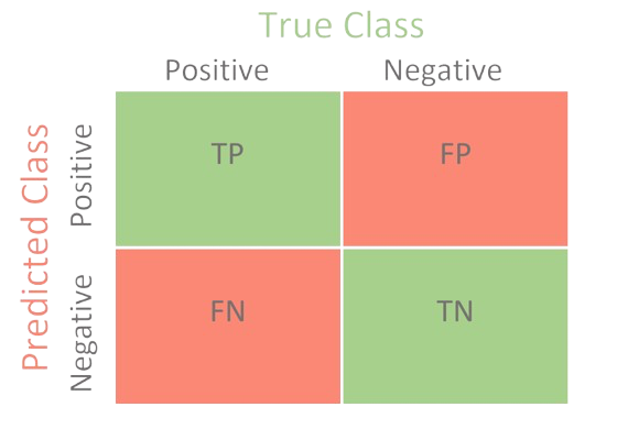
Most fairness metrics for discrete prediction algorithms use some combination of true positives, true negatives, false positives, and false negatives in their calculations. A helpful way of visualizing the difference between terms is through a confusion matrix (like the one depicted for a binary prediction algorithm in Figure 2). Notice how true positives, true negatives, false positives, and false negatives all rely on comparing an observation’s predicted class to its true (or actual) class. Specifically, a true positive (TP) is when observation’s true class and predicted class are both positive, and a false positive (FP) is when the observation’s true class is positive but its predicted class is not. On the other hand, a true negative (TN) is when observation’s true class and predicted class are both negative, and a false negative (FN) is when the observation’s true class is positive but its predicted class is not.
An Real-World Example: The Correctional Offender Management Profiling for Alternative Sanctions (COMPAS) algorithm is used in US courtrooms to assess the likelihood of a defendant becoming a recidivist (i.e. being re-convicted) by assigning each defendant a score between 1-10 based on their predicted likelihood of recidivism. A defendant is considered to have a low risk of recidivism if their COMPAS score is between 1-4 and medium to high risk of recidivism if their COMPAS score is between 5-10. In ProPublica’s seminal analysis of COMPAS, true positives, false positives, true negatives, and false negatives would be defined as follows:1
- A true positive is when a defendant receives a COMPAS score between 5-10 and is re-convicted in the two years after they were scored.
- A false positive is when a defendant receives a COMPAS score between 5-10 but is not re-convicted in the two years after they were scored.
- A true negative is when a defendant receives a COMPAS score between 1-4 and is not re-convicted in the two years after they were scored.
- A false negative is when a defendant receives a COMPAS score between 1-4 but is re-convicted in the two years after they were scored.
1.2 Conditional Probability
Another important concept to understand when talking about statistical fairness metrics is conditional probability which is the probability of an event given that some other event occurs. For example, let A and B be two events, where B has a non-zero probability of occurring, then the conditional probability of A given B (i.e. \mathbb{P}(A|B)) can be calculated as follows:
\mathbb{P}(A|B) = \frac{\mathbb{P}(A\cap B)}{\mathbb{P}(B)}
In real-life cases, we rarely know the true probability of events occurring. Instead, we must estimate this probability empirically from a sample. For instance, we can find the proportion of times that both event A and event B occurred out of the total number of times that event B occurred in our sample.
Oftentimes, in the context of outcome-based algorithmic fairness metrics, the relevant conditional probabilities are computed by comparing the true positives, false positives, true negatives, and/or false negatives between the relevant groups within a sample.
2 Algorithmic Fairness Metrics
2.1 Equal Accuracy
Perhaps the most flat-footed algorithmic fairness metric is Equal Accuracy, which says that an algorithm is unfair if it has unequal accuracy across relevant groups. That is, suppose we had two relevant groups, denoted as A and B. Then, according to Equal Accuracy, an algorithm is unfair if:2
\mathbb{P}(\mathrm{Pred.~Class = True~Class~|~Group = A}) \neq \mathbb{P}(\mathrm{Pred.~Class = True~Class~|~Group = B}) In other words, an algorithm is unfair when the probability that the predicted class is the same as the true class is different between relevant groups under the Equal Accuracy metric.
2.2 Predictive Parity (sometimes called Equal Opportunity)
However, depending on the context in which the algorithm is used, it might be crucial from the perspective fairness to ensure that there is equal accuracy between groups among those predicted as part of the positive class, rather than simply guaranteeing that there is equal accuracy between the relevant groups in general (i.e., unconditioned on the individual’s predicted class). For instance, it seems more important from the perspective of fairness that a hiring algorithm correctly identify the same proportion of candidates who are qualified for a job between relevant groups than that the same proportion of candidates are correctly identified as being unqualified between relevant groups.
The metric of Predictive Parity captures this concern. According to Predictive Parity, an algorithm is unfair between relevant groups A and B if:
\mathbb{P}(\mathrm{True~Class = 1|~Pred.~Class =1,~Group = A}) \neq \mathbb{P}(\mathrm{True~Class = 1|~Pred.~Class = 1,~Group = B}) Notice how Predictive Parity relates to the algorithm’s Positive Predictive Value (PPV) or Precision. Specifically, when an algorithm satisfies Predictive Parity, we expect for the PPV and Precision for the relevant groups to be equal. That is:
\left( \frac{TP + FN}{TP + FP} \right)_\mathrm{Group~=~A} = \left( \frac{TP + FN}{TP + FP} \right)_\mathrm{Group~=~B} Sometimes, Predictive Parity is called the Equal Opportunity metric.
2.3 Equal False Positive Rates
Like the Predictive Parity metric, the Equal False Positive Rates metric only equalizes prediction performance among a subset of individuals in the relevant groups. Per the Equal False Positive Rates metric, an algorithm is unfair if the probability that an individual whose true class is negative is predicted as positive differs between the relevant groups. This can be formalized as:
\mathbb{P}(\mathrm{Pred.~Class = 1|~True~Class = 0,~Group = A}) \neq \mathbb{P}(\mathrm{Pred.~Class = 1|~True~Class = 0,~Group = B})
For example, using Equal False Positive Rates as a fairness metric would prevent cases where more people in group A are incorrectly identified as recidivists than in group B. In the ProPublica report on the COMPAS algorithm, ADD argue COMPAS is biased, and thus unfair, on the basis on unequal false positive rates between Black and White defendants. Specifically, they found that Black defendants were two times more likely to be falsely labeled as future criminals than white defendants.
2.4 Equal False Negative Rates
Along a similar vein to Equal False Positive Rates is the fairness metric of Equal False Negative Rates, which says that an algorithm is unfair if the probability that an individual whose true class is negative will be predicted as positive differs between relevant groups:
\mathbb{P}(\mathrm{Pred.~Class = 0|~True~Class = 1,~Group = A}) \neq \mathbb{P}(\mathrm{Pred.~Class = 0|~True~Class = 1,~Group = B})
ADD also found that COMPAS had different false negative rates between Black and white defendants. Namely, “white defendants were mislabeled as low risk more often than black defendants”, which they also used to justify their conclusion that the COMPAS algorith was biased and thus unfair CITE.
2.5 Equal Ratios of False Positive Rates to False Negative Rates
A looser requirement for algorithmic fairness is Equal Ratios of False Positive Rates to False Negative Rates, which does not require either Equal False Positive Rates or Equal False Negative Rates to hold between relevant groups. Putting together the formalizations of the two prior metrics, we get that an algorithm is unfair, according to Equal Ratios of False Positive Rates to False Negative Rates, if:
\frac{\mathbb{P}(\mathrm{Pred.~Class = 1|~True~Class = 0,~Group = A})}{\mathbb{P}(\mathrm{Pred.~Class = 0|~True~Class = 1,~Group = A})} \neq \frac{\mathbb{P}(\mathrm{Pred.~Class = 1|~True~Class = 0,~Group = B})}{\mathbb{P}(\mathrm{Pred.~Class = 0|~True~Class = 1,~Group = B})}
At first glance, it is hard to understand why would care about equal ratios of false positive rates to false negative rates; would it not make more sense to want both equal false positive rates and equal false negative rates to hold between relevant groups? One reason that we might care about Equal Ratios of False Positive Rates to False Negative Rates for algorithmic fairness is because we care about the algorithm ADD
2.6 Demographic/Statistical Parity
\mathbb{P}(\mathrm{Pred.~Class = 1~|~Group = A}) \neq \mathbb{P}(\mathrm{Pred.~Class = 1~|~Group = B})
2.7 Equalized Odds
\mathbb{P}(\mathrm{Pred.~Class = 1|~True~Class = X,~Group = A}) \neq \mathbb{P}(\mathrm{Pred.~Class = 1|~True~Class = X,~Group = B}) where, X \in \{0,1\}
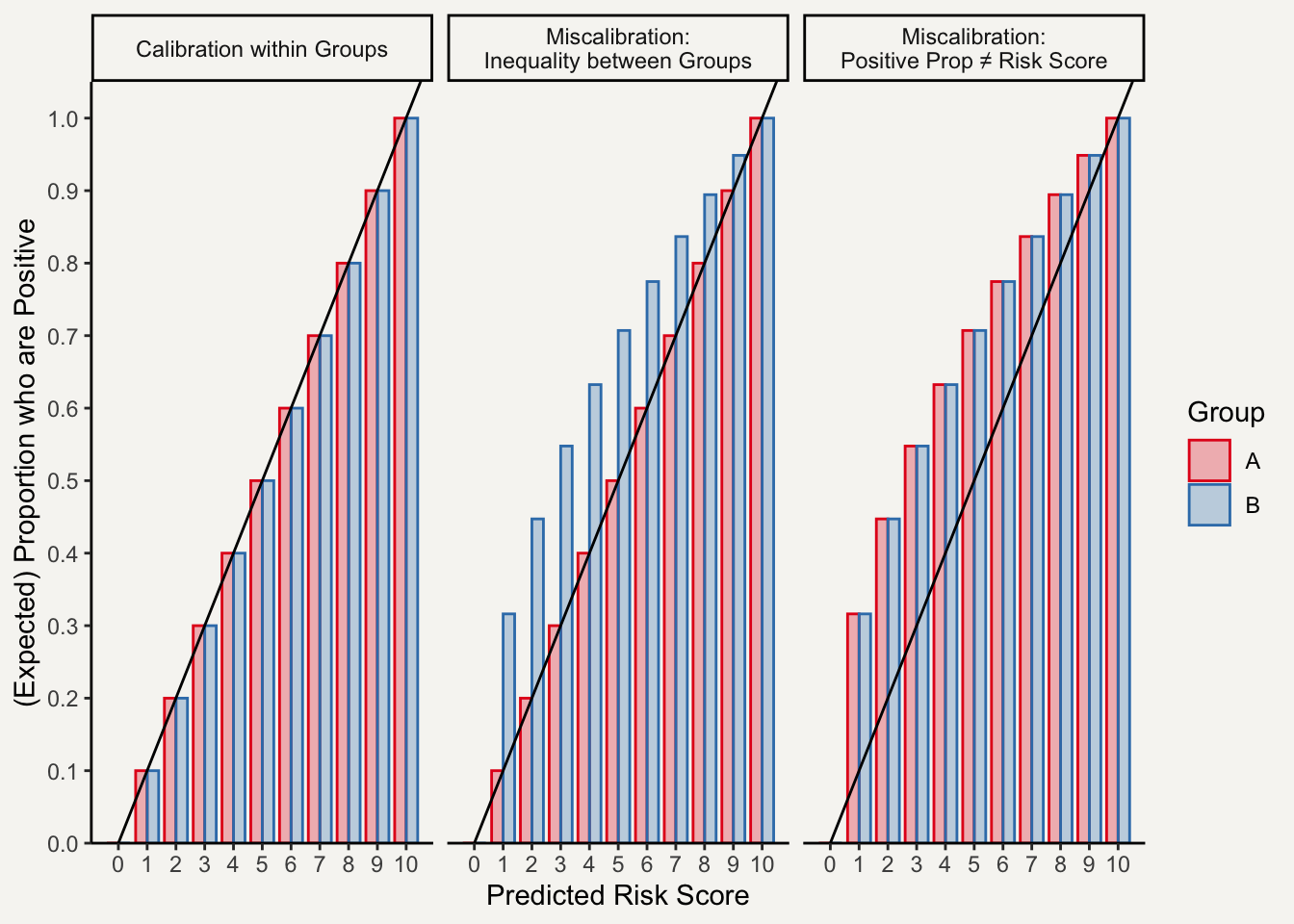
2.8 Calibration within Groups
Calibration within Groups is a metric specifically for algorithms that output risk scores, i.e., an ordinal prediction for each observation that represents the probability that it belongs to the positive class. The COMPAS algorithm is a canonical example of a risk score algorithm in the algorithmic fairness literature.
Per Calibration within Groups, an algorithm is fair if for each possible risk score, the (expected) proportion of individuals assigned that risk score who are actually members of the positive class is equal to the risk score and the same for each relevant group. That is:
\mathbb{P}(\hat R \mid \mathrm{True~Class} = 1, \mathrm{~Group} = X) = \hat R
where, X \in \{A,B, \dots\} and \hat R denotes predicted risk score, possibility transformed to be between 0 and 1 (inclusive).
Since there are several moving parts for satisfying Calibration within Groups metric, it is perhaps easier to understand through toy examples (see Figure 3).
One motivation for Calibration within Groups is that ADD.
2.9 Balance for Positive Class
Alternatively, we might be most concerned with disparate performance of risk score algorithms on individuals who are members of the positive class.
According to the Balance for Positive Class metric, an algorithm is unfair if the expected risk score assigned to individuals who are actually members of the positive differs across relevant groups:
\mathbb{E}[\hat R \mid \mathrm{True~Class} = 1, \mathrm{~Group = A}]= \mathbb{E}[\hat R \mid \mathrm{True~Class} = 1, \mathrm{~Group = B}]
2.10 Balance for Negative Class
The (expected) average risk score assigned to those individuals who are actually members of the negative class is the same for each relevant group:
\mathbb{E}[\hat R \mid \mathrm{True~Class} = 0, \mathrm{~Group = A}]= \mathbb{E}[\hat R \mid \mathrm{True~Class} = 0, \mathrm{~Group = B}]
3 Concerns with Outcome-Based Fairness Metrics
3.1 Impossibility Results
One of the largest concerns in the Statistics and Machine Learning communities with outcome-based algorithmic fairness metrics is that it has been mathematically proven that three intuitively appealing outcome-based metrics for algorithmic fairness – (1) calibration within groups, (2) equal false positive rates, and (3) equal false negative rates – cannot be simultaneously satisfied when the base rates (i.e., the rate of positive instances) differ between the relevant groups (see Kleinberg, Mullainathan, and Raghavan (2016), Chouldechova (2017), and CITE). These results are often referred to as Impossibility Results for algorithmic fairness.
A natural conclusion given the impossibility results is that algorithmic fairness is not possible when the base rates differ between relevant groups, which will be the case when there is pre-existing injustice, such as in bank lending, credit scores, hiring, education, and the criminal justice system. However, it is important to note that this conclusion relies on a hidden premise that all three of these outcome-based algorithmic fairness metrics – (1) calibration within groups, (2) equal false positive rates, and (3) equal false negative rates – all accurately capture the concept of fairness.
However, I would argue that …ADD
3.2 Defining “Revelant Groups”
Group-based fairness metrics (which includes all of the ones that I outline in this notebook) also require a condition to hold among “relevant groups”. In practice, “relevant groups” is treated as synonymous with groups that correspond to federally protected characteristics, which include race, color, religion, sex, sexual orientation, disability status, and age.3
However, what identity group is “relevant” might change between contexts. Indeed, Lazar and Stone (2023) note that from the perspective of algorithmic justice, we care about comparing the model’s performance for “systematically disadvantaged groups” against that for “systematically advantaged groups” (see their Prioritarian Performance Principle), where a social ontology is needed to determine the relative social position of groups in a given context. This social ontology is often quite complicated in practice – reflecting that real-life social positions tend to be both complex and intersectional. For example, suppose we were trying to assess whether an hiring algorithm is unfair ADD.
Hence, group-based fairness metrics require us to define “socially salient” groups – often in a way that obfuscates the complexities of social positions for the sake of …ADD.
References
Chouldechova, Alexandra. 2017. “Fair Prediction with Disparate Impact: A Study of Bias in Recidivism Prediction Instruments.” Big Data 5 (2): 153–63. https://doi.org/10.1089/big.2016.0047.
Kleinberg, Jon, Sendhil Mullainathan, and Manish Raghavan. 2016. arXiv. https://doi.org/10.48550/ARXIV.1609.05807.
Lazar, Seth, and Jake Stone. 2023. “On the Site of Predictive Justice.” Noûs 58 (3): 730–54. https://doi.org/10.1111/nous.12477.
Footnotes
From the COMPAS example, we can already see a point of contention in characterizing algorithmic fairness for discrete prediction problems, which is what threshold to use for decision-making? For example, why separate low from medium to high risk of recidivism at 4-5 rather than 3-4 or 5-6? How do we think about fairness when determining decision thresholds?↩︎
In this notebook, I interpret each fairness metric as a necessary but not necessarily sufficient condition of algorithm fairness, meaning that an algorithm would be considered unfair if it does not satisfy X metric necessary for algorithmic fairness but it would not necessarily be fair if it does satisfy the required metric. This, in my opinion, is the most charitable way of interpreting the common statistical fairness metrics that I discuss in this notebook.↩︎
For more information, see https://civilrights.osu.edu/training-and-education/protected-class-definitions.↩︎